Plasticity Without Forgetting

Learner 1.0 at two capacities against capacity-matched LoRA on a four-domain continual-learning stream.

Does the protection cost you the learning? Can a method learn a stream of new domains as well as a strong weight-update method, while actually keeping them?

Conclusions

Three results carry this study.

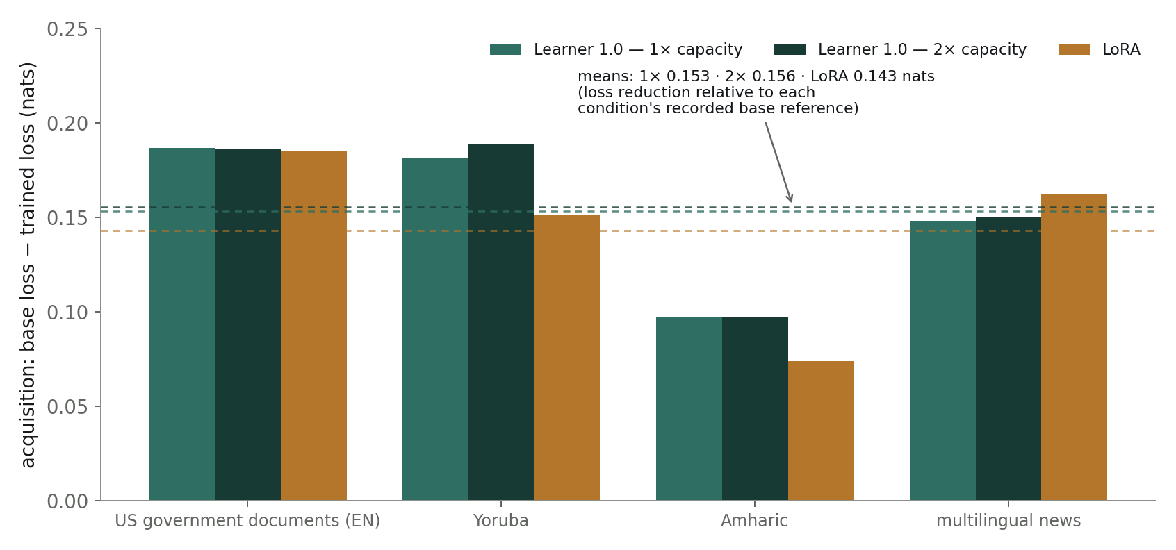
One. Learner 1.0 learned at least as much as the rank-matched LoRA, and kept it. Averaged over the four domains it ends with more loss reduction than LoRA — 0.153 nats at 1× and 0.156 at 2× against LoRA’s 0.143 — ahead in three of the four domains and behind in news. Over the same stream LoRA’s earlier domains lost +0.070, +0.060 and +0.034 nats while Learner 1.0’s moved by thousandths. The plasticity did not cost the retention, and the retention did not cost the plasticity. Acquisition →

Two. At the first evaluation, after 25 updates per domain, Learner 1.0 showed 82–125% of LoRA’s 300-update loss reduction, measured from each condition’s recorded base reference. Twenty-five updates are 8.3 per cent of a domain’s 300. By domain the figures are 93 and 90 per cent on the first domain at 1× and 2×, 109 and 110 on Yoruba, 125 and 124 on the language domain, and 82 and 85 on news, the one domain LoRA ends ahead on. On two of the four it had already passed LoRA’s end point outright. The evaluation grid is every 25 updates, so 25 is a ceiling on when this happened, not a measurement of when. Curve shape →

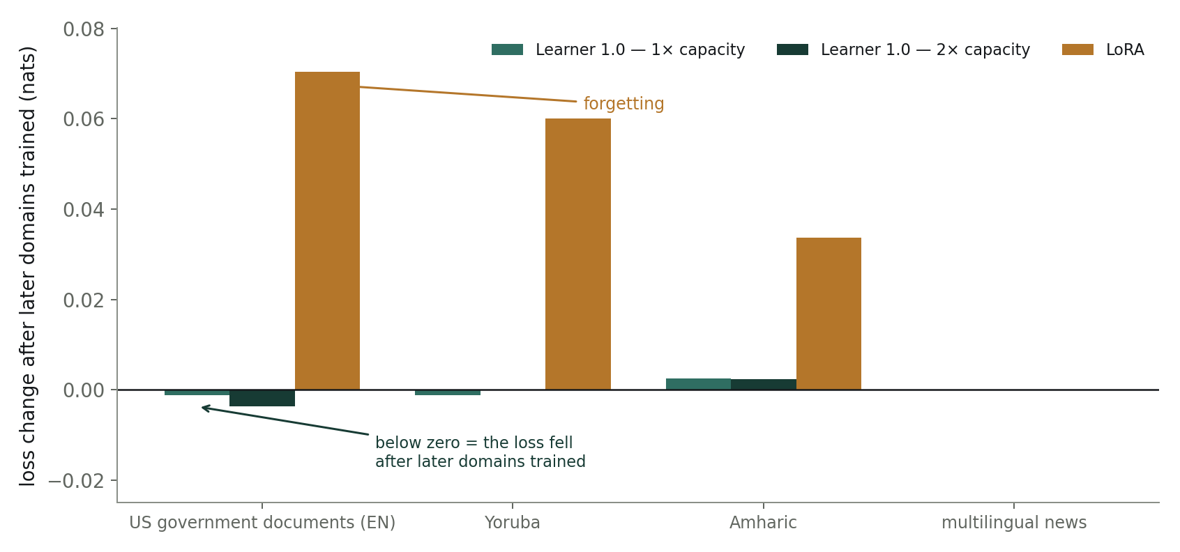
Three. Earlier domains improved while later ones trained. That is positive backward transfer, the sought-after direction: the later material reuses what the earlier material built instead of overwriting it. At 1× the first two domains fell by 0.0011 and 0.0012 nats after their own training was over, and at 2× the first fell by 0.0037. The third rose by 0.002 in both. The effect is small and each experiment is one run. Forgetting →

Seven findings follow, one per section. Each links to the section that measures it.

On the same four-domain stream, LoRA forgot and Learner 1.0, at both capacities, did not. Re-measured at the end of the stream, LoRA's earlier domains had lost +0.070, +0.060 and +0.034 nats. Learner 1.0 (1×)'s changed by −0.001, −0.001 and +0.002. Learner 1.0 (2×)'s changed by −0.004, −0.000 and +0.002. Every earlier domain was retained within a few thousandths of a nat. The mean change was +0.0001 nats at 1× and −0.0005 at 2×. Forgetting →
No experiment is told where one domain ends and the next begins. Data arrives as one uninterrupted stream: a single uninterrupted stream of 1,200 steps with no task identifiers and no boundary signal of any kind. Whatever each method does about interference, it does blind. Setup →
Retention did not come with less measured acquisition. Acquisition here is each experiment’s loss reduction from its own recorded base reference, so it is not a matched measure of learning during the stream alone. On that measure, both Learner 1.0 experiments end their domains with slightly more loss reduction than LoRA on average: 0.153 (1×) and 0.156 (2×) vs 0.143 nats. They are ahead in three domains and behind in news. And At the one higher rate tried for this LoRA configuration, 10× (2×10⁻⁴), it diverged. It ends 0.93 nats worse than the base model on the very domain it was training (§7). Acquisition →
This LoRA configuration was tried at two learning rates, and at the higher one it diverged. At 2×10⁻⁴ it ends +0.93 nats above the base model on the domain it was training, which is why the comparison runs it at 2×10⁻⁵. Learner 1.0 ran at 1×10⁻³. Two rates are a trial, not a sweep, and they say nothing about other adapter setups. The learning-rate axis →
Doubling Learner 1.0's capacity bought almost nothing. Going from 1.14B to 2.28B trainable parameters moved mean acquisition by +0.002 nats and left retention where it was (~zero). Neither the learning nor the retention at 1× looks capacity-limited on this stream. Doubling capacity →
The Learner 1.0 curves are nearly flat from the first measurement. At the first recorded evaluation, 25 steps into the displayed stream, both Learner 1.0 experiments are already close to their eventual loss on the first domain, while LoRA descends across the 300 steps. The plotted interval does not isolate how much of the improvement from the base reference was produced during those 25 steps. Curves inside each domain →
The never-trained control did not get worse. A 64-window bank that no experiment trains on, mostly Amharic text with no window in common with the Amharic domain, moved by about 0.01 nats across the stream under Learner 1.0 (8 windows measured) and ended 0.084 nats below its starting value under LoRA (all 64 windows). The never-trained control →

Introduction

Adapting a large language model to new material usually means choosing between two failure modes. Full fine-tuning and its parameter-efficient variants learn the new material well, but when the material arrives sequentially, one domain after another, the way real usage arrives, each new domain overwrites some of what came before. The standard mitigation is to avoid the sequential setting altogether: mix everything and retrain. That works for a lab. It does not work for a system that must keep learning after it ships.

Learner 1.0 is built for exactly that sequential setting: a fixed set of trainable parameters is added to the base model. The mechanism itself is proprietary and is not described here. This post measures the question above directly, on one base model and one data stream, with three experiments: Learner 1.0 at a trainable capacity matched to LoRA's to within 3% (henceforth Learner 1.0 (1×)), Learner 1.0 at double that capacity (Learner 1.0 (2×)), and rank-256 LoRA. The 2× experiment answers a second question the matched pair cannot: is what you see at 1× capacity-limited, or a property of the architecture?

Setup: one base model, one stream, three experiments

The base model is Learner 1.0 in bf16, identical across all three experiments. The stream is four text domains trained strictly in sequence: English-language US government documents (congressional reports and hearing transcripts), Yoruba, Amharic, and multilingual news articles. Each gets 300 optimizer steps on 256-token windows, 1,200 steps total, on the same training windows and in the same domain order for all experiments.¹ Each domain holds out 8 windows that are never trained. A fifth set of 64 windows (held_control), 59 of them Amharic text with no window in common with the Amharic domain, is never trained by any experiment and exists to check text near the stream that no experiment trained. The Learner 1.0 experiments were scored on 8 of its windows after every domain; the LoRA experiment was scored on all 64 before and after the stream. All losses are next-token cross-entropy in nats on those held-out windows. Acquisition is the loss reduction from each condition’s recorded base reference. Backward transfer is final loss minus own-end loss on the same held-out windows.

The training unit. Training proceeds one example at a time: batch size 1, with no gradient accumulation across examples. Each example is one 256-token text window. The model predicts each next token, so a window supplies 255 prediction targets, and the parameters are updated once after every window. This holds for all three experiments. A domain is 300 windows, so 300 updates, 76,800 input tokens and 76,500 next-token targets; the stream is 1,200 updates, 307,200 input tokens and 306,000 targets.

Two real training windows. Each is an excerpt from a 256-token training window, decoded from the token sequence that was trained.

includes $260 million for Public Health Infrastructure and Capacity Grants (PHIG) to continue to address gaps in core public health capacity and infrastructure at the state, tribal, territorial, and local levels. PHIG's groundbreaking, flexible model lets health department recipients invest in the people, services, and systems that can address their communities' most pressing needs.
Domain 1, training window 151 of 300. Source: a congressional hearing record published on GovInfo, a work of the US Government.

Wọ́n bíi sínú Jrāwa Zenata àwọn ẹ̀yà ìbẹ̀rẹ pẹ̀pẹ̀ 7th century. Fún ọdún gbáko ni ó fi darí ìpínlẹ̀ Berber tí ó ní ìyánǹda láti Aurès Mountains náà lọ sí ilẹ̀ olómi nínú aginjù Gadames (ní 695–700 AD).
Domain 2, training window 41 of 300. Source: the Yoruba Wikipedia article on Al-Kahina, CC BY-SA 4.0, Wikipedia contributors.

The training data. Every window that was trained or measured is in the replication repository, in science/plasticity-without-forgetting/data: 1,200 training windows, 32 held-out windows and the 64-window control. Each row gives the exact token ids that were executed and the text decoded from them. The rows are in the order the Learner 1.0 experiments trained them. You can read them in the sample viewer, or open the files:

US government documents: 300 training windows, 8 held-out windows
Yoruba: 300 training windows, 8 held-out windows
Amharic: 300 training windows, 8 held-out windows
Multilingual news: 300 training windows, 8 held-out windows
Never-trained control: 64 windows (no training rows)

The Yoruba, Amharic, news and control text comes from third-party sources. It is held under those sources’ own terms. The repository gives the dataset and pinned revision each set was cut from. It does not have a record of which article or page each window came from. The files are for inspection; the repository does not run this training.

There are no task boundaries. Much of the continual-learning literature quietly assumes the opposite. No experiment receives any signal that a domain has ended or a new one has begun: no task identifiers and no task-boundary signal. Each experiment runs as one uninterrupted training stream of 1,200 steps. From the learner's point of view there is only a stream of batches whose statistics happen to change. Every forgetting and retention number below is measured under that blindness.

	Learner 1.0 (1×)	Learner 1.0 (2×)	LoRA
base model	Learner 1.0, bf16, 64 layers
method	proprietary (details withheld). The two experiments differ only in trainable capacity		rank-256 adapters on all three MLP projections; update ΔW = B·A
trainable parameters	1.14 billion (fp32)	2.28 billion (fp32)	1.11 billion (0.97× of Learner 1.0 (1×))
learning rate	1×10⁻³ (stream)		2×10⁻⁵. 2×10⁻⁴ was tried first and diverges (§7)
input protocol	one window per update, in one uninterrupted stream per experiment. No task identifiers or task-boundary signal supplied
stream	the same windows and domain order: 4 domains × 300 steps × 256-token windows
batch size	1 window per update, no gradient accumulation
samples and updates	300 per domain, 1,200 per stream
input tokens	76,800 per domain, 307,200 per stream
next-token targets	76,500 per domain, 306,000 per stream (255 per window)
domain interleaving	none: the four domains are trained strictly one after the other in every experiment

The capacity-matched comparison is Learner 1.0 (1×) vs LoRA: 1.141B vs 1.107B trainable parameters, a 0.97× match. The 2× experiment is deliberately not matched: it exists to test whether the 1× results are sitting against a capacity ceiling, and every claim of parity or superiority over LoRA below is made from the 1× experiment.

Forgetting: the headline difference

Figure 1 shows the entire experiment at once. Each panel walks the same stream left to right: faint line, per-step training loss. Dotted line, held-out validation loss measured every 25 steps. Dashed black line, the recorded base-reference loss on that domain. The three panels share identical axes, so every loss is directly comparable. The part to read is the right edge: after the last domain finishes, every earlier domain is re-evaluated, and the diamond shows where it landed.

Learner 1.0 at two capacities vs LoRA across the four-domain stream — **Figure 1.** All three experiments learn every domain. Only LoRA loses the earlier ones by the end. All three experiments drive each domain's held-out loss below the base model (dashed black) while training on it. The difference is what happens afterward: LoRA's earlier domains, re-measured at the end (hollow diamonds), have risen +0.070, +0.060 and +0.034 nats above where their own training left them. That is the classic signature of catastrophic forgetting, largest for the domain trained longest ago. Both Learner 1.0 panels put their diamonds on the line (worst single-domain drift +0.0025 at 1×, +0.0024 at 2×), and doubling the capacity changes nothing about the shape. Same base model, same data, same step budget, and no experiment told where the domains switch. Redrawn from the released receipts by the repository’s own plot code as Figure 8.

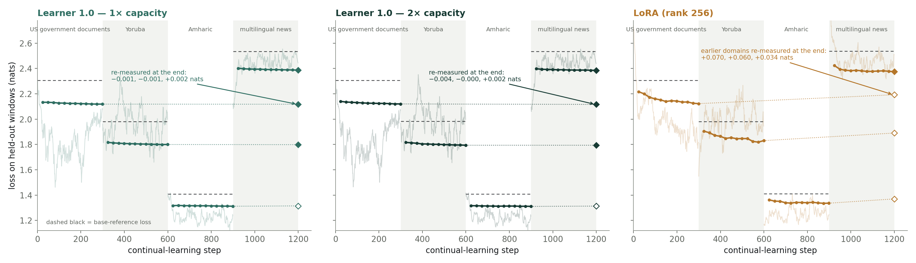
Figure 2 isolates the end-of-stream change per domain, the quantity usually reported as backward transfer, where positive means the domain got worse after later training. LoRA's forgetting is ordered exactly as interference predicts: the earliest domain forgets the most. The Learner 1.0 bars hover at zero in both experiments, and several are negative. After the later domains trained, those losses were slightly lower (the first two at 1×, and the first domain most strongly, −0.004, at 2×). Averaged over the three earlier domains, LoRA forgets 0.0547 nats, Learner 1.0 (1×) +0.0001, and Learner 1.0 (2×) −0.0005. That is drift five hundred times smaller than LoRA's at 1×, and net-negative at 2×.

Backward transfer per domain, three arms — **Figure 2.** Every LoRA domain lost ground, every Learner 1.0 domain held within ±0.004 nats. Change in each domain's held-out loss between the end of its own training and the end of the stream. Every LoRA bar is positive (forgetting), ordered by how long ago the domain was trained. Every Learner 1.0 bar, at either capacity, is within ±0.004 of zero. And the negative bars are positive backward transfer, not merely the absence of forgetting. Learner 1.0's worst single-domain drift (+0.0025 at 1×) is 28× smaller than LoRA's (+0.0703). Redrawn from the released receipts by the repository’s own plot code as Figure 10.

The effect does not come from having more room to write into. LoRA's rank-256 update is one shared subspace that every domain must rewrite. The method Learner 1.0 uses instead is withheld. That the retention numbers are indistinguishable at 1× and 2× capacity is itself evidence for this reading: interference-driven forgetting should ease as capacity grows, but there is no forgetting left to ease.

Sequential training has produced this signature since 1989, and the usual ways of suppressing it buy retention by giving something up: a boundary signal, a replay buffer, or a parameter count that grows with the task list. This stream supplies none of the three.

If a model can take a new domain without disturbing the ones already in it, retraining from mixed data stops being the only safe way to ship an update. Domains can then arrive in whatever order your users produce them.

Replicate it. Receipts and curves for this figure: science/plasticity-without-forgetting in the replication repository

Acquisition: protection is not paid for in learning

Protection would be uninteresting if it were bought with plasticity. Figure 3 shows acquisition: how many nats each experiment removes from the base model's loss on a domain's held-out windows by the end of that domain's training. Both Learner 1.0 experiments acquire more than LoRA in three domains and tie in the fourth. Averaged over the stream they remove 0.153 (1×) and 0.156 (2×) nats to LoRA's 0.143. The protection is not paid for in learning.

Acquisition per domain, three arms — **Figure 3.** Loss reduction relative to each base reference. Loss reduction relative to the recorded base reference, per domain (higher is better), measured on held-out windows at the end of each domain's own training. Both Learner 1.0 experiments (teals) edge out LoRA in government documents, Yoruba and Amharic and trail it in news (0.148 and 0.150 vs 0.162). Means are 0.153 / 0.156 vs 0.143 nats. The two teal bars are nearly equal in every domain. Doubling Learner 1.0's capacity buys almost nothing, which says acquisition at 1× is not capacity-limited. The measured acquisition is similar across the three; the difference is in retention. Each bar is taken from that experiment’s own base reference, so this is not a matched comparison of learning during the stream alone.

Retention is easy to buy by learning less: a method that barely moves has little to lose. The question that decides whether the protection is worth anything is whether the protected experiment still learns as much as the unprotected one on the domain in front of it.

Parity of acquisition means the retention property costs nothing at the point of use. You can take it and still have the stronger model on the domain you are training right now.

Replicate it. Receipts and curves for this figure: science/plasticity-without-forgetting in the replication repository

Doubling capacity: what it buys, and what it doesn't

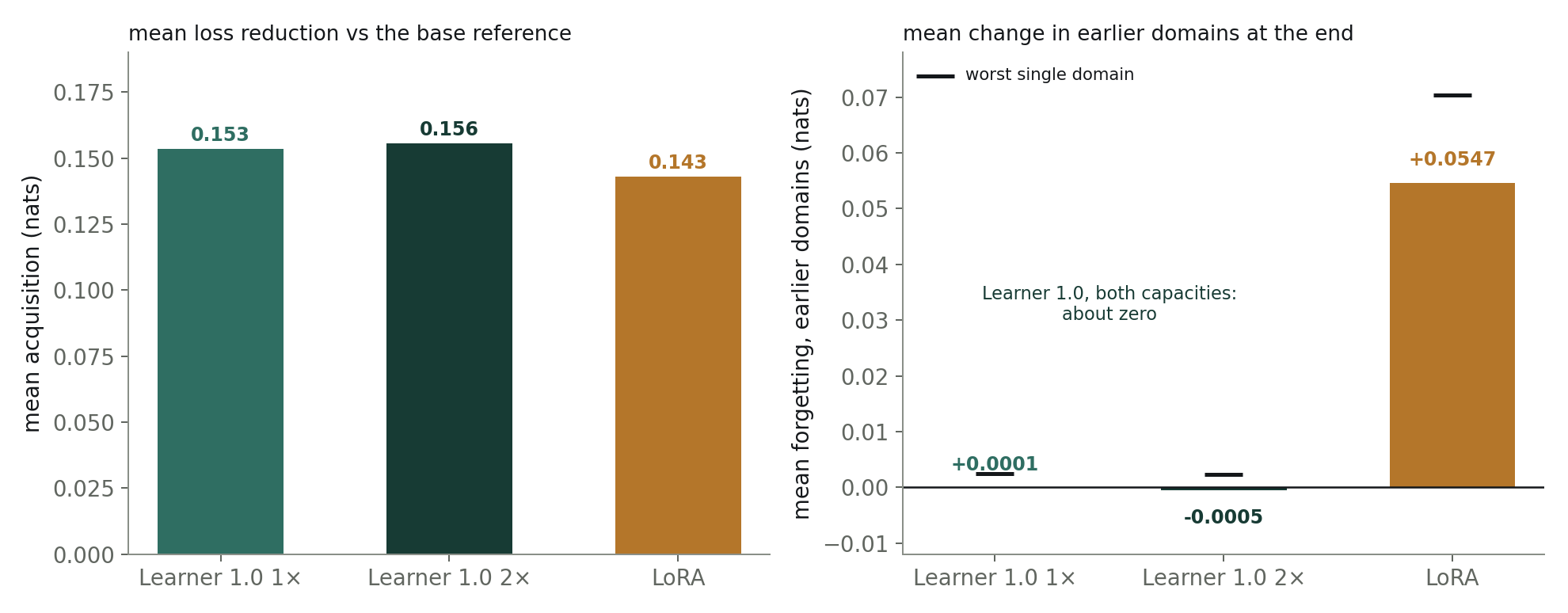
The 2× experiment exists to answer one question: are the 1× results capacity-limited? Figure 4 puts the two summary quantities side by side for all three experiments: mean acquisition on the left, mean forgetting on the right. The answer is no, twice over. Doubling the trainable parameters from 1.14B to 2.28B moves mean acquisition from 0.153 to 0.156 nats, a 2% change on a 100% capacity increase. Retention, already at ~zero, has nowhere to go (mean drift +0.0001 → −0.0005, worst single domain +0.0025 → +0.0024).

Mean acquisition and mean forgetting, three arms side by side — **Figure 4.** Both Learner 1.0 capacities show slightly more mean loss reduction than LoRA and carry 500× less drift. Left: mean acquisition across the four domains (higher is better). Right: mean forgetting across the three earlier domains (lower is better, with the black dash marking each experiment's worst single domain). Both Learner 1.0 capacities show slightly more mean loss reduction than LoRA, relative to the base reference, and forget ~nothing. LoRA carries 500× the drift. The near-identical teal pairs in both panels are the capacity result: neither Learner 1.0's learning nor its retention moves when the parameter budget doubles.

A result that appears at exactly one parameter budget is a tuning artefact until it is shown at another. Doubling the budget is the cheapest test of whether a number is a property of the design or of its size.

At this stream length and per-domain budget, the binding constraint on Learner 1.0's acquisition is not parameter count.

Replicate it. Receipts and curves for this figure: science/plasticity-without-forgetting in the replication repository

The learning-rate axis: why LoRA sits at 2×10⁻⁵

The setup table contains an asymmetry that deserves the same scrutiny as capacity: Learner 1.0's stream learning rate is 50× LoRA's. Could LoRA not simply be run hotter and learn more? It was tried. The 2×10⁻⁵ rate was itself selected by that trial. The comparator was fixed in advance to run first at 2×10⁻⁴, the rate an earlier reference run had used, on exactly the same stream (the domain windows are byte-identical between the two runs, and only the learning rate differs). Figure 5 shows what happened.

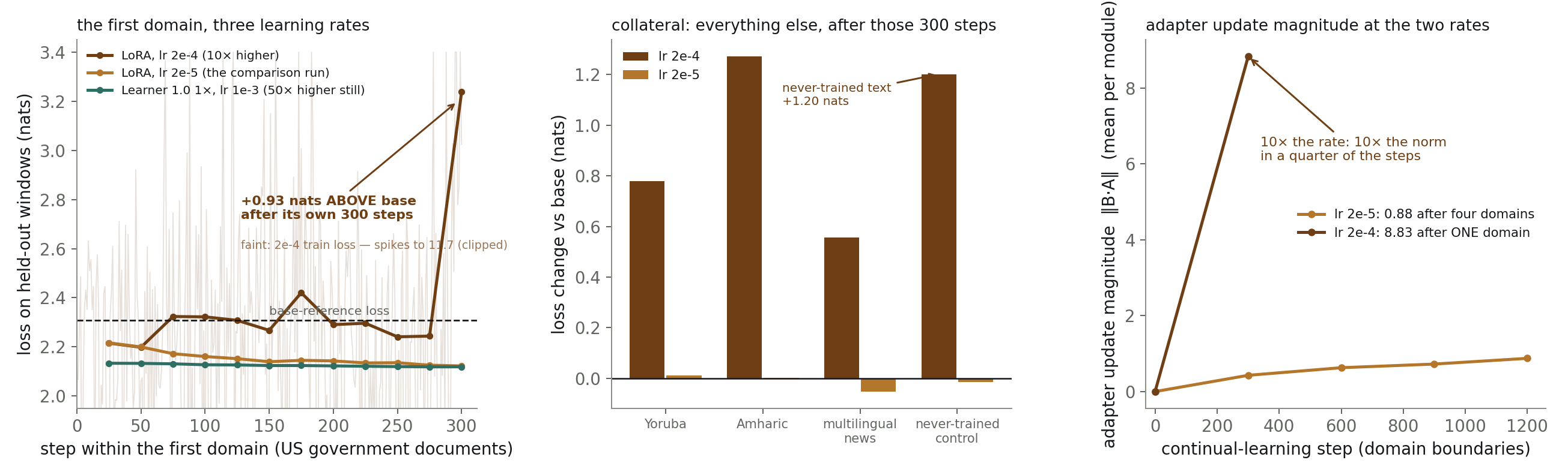
LoRA learning-rate ablation: 2e-4 diverges — **Figure 5.** One decade up the learning-rate axis, LoRA diverges. Left: held-out loss on the first domain during its own 300 training steps. At 2×10⁻⁴ (dark), LoRA learns briefly (2.20 at step 50, below the base model) and then destabilizes, ending +0.93 nats *above* base on the domain it was training. Its train loss (faint) spikes to 11.7 along the way. At 2×10⁻⁵ (amber) it descends normally. Learner 1.0 (teal) ran at 1×10⁻³. Middle: after those 300 steps, the 2×10⁻⁴ run has damaged every other domain by +0.56 to +1.27 nats, including text that was never trained (+1.20). At 2×10⁻⁵ every other column is within ±0.05. Right: the adapter's update magnitude ‖B·A‖ reaches 8.83 after *one* domain at 2×10⁻⁴ versus 0.88 after all *four* at 2×10⁻⁵.

2×10⁻⁵ is where this LoRA configuration works. At 2×10⁻⁴ it diverged. Learner 1.0 ran at 1×10⁻³ on the same one-window updates, with no task-boundary signal, and produced Figures 1–3.

The run at 2×10⁻⁴ was stopped by a runtime guard at the first domain boundary: its acquisition on the domain it had just trained was negative, and a stream continued past that point measures damage, not forgetting. The mechanism is visible in the right panel and is a property of the adapter, not of the data: LoRA's weight update is the product of two trained matrices, applied here at the least-damped scaling (α/r = 1), and its magnitude has no ceiling. A tenfold learning-rate increase produced a roughly tenfold larger update surface in a quarter of the steps, . Weight decay and data ordering were both eliminated as causes (the diverging run used weight decay 0 and within-domain shuffling, reproducing the divergence measured earlier under other settings).

The width of the stable learning-rate window is part of what you are choosing between. A comparison is only as fair as the tuning given to the experiment that loses it. This one tried the LoRA configuration at two rates, which is a trial and not a sweep.

Replicate it. Receipts and curves for this figure: science/plasticity-without-forgetting in the replication repository

Learning curves inside each domain

Figure 6 plots the three experiments together inside each domain's 300-step window, with the recorded base reference drawn as a dashed level. The shape difference is consistent: at the first recorded evaluation, 25 steps into each domain, both Learner 1.0 experiments are already close to their eventual loss, and then flatten. The plotted interval does not isolate how much of the improvement from the base reference was produced during those 25 steps. LoRA approaches its final loss gradually across the window. In three of the four domains the Learner 1.0 curves are below LoRA's at every measured step. In news they cross and LoRA finishes marginally lower.

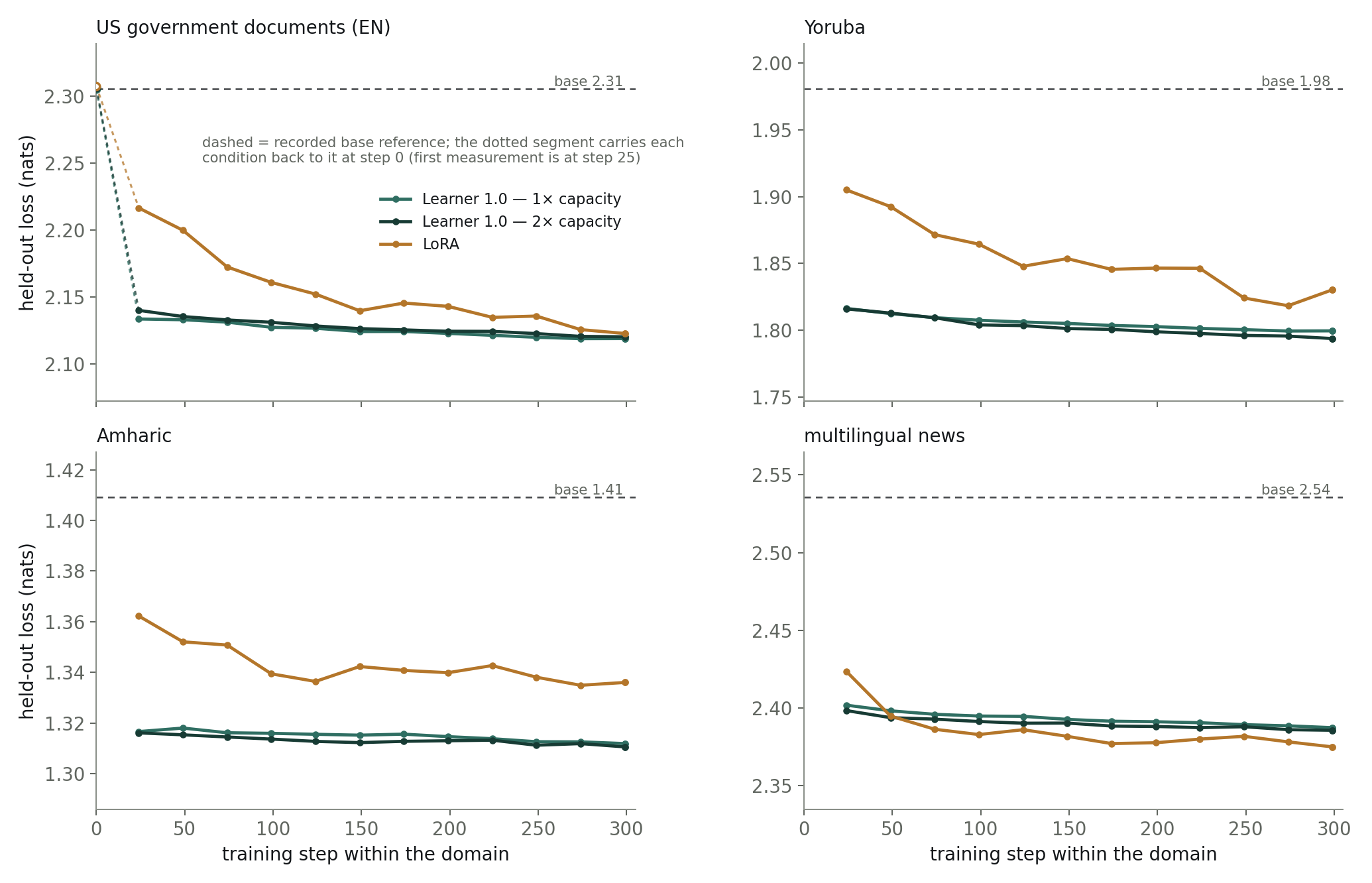
Within-domain learning curves, three arms — **Figure 6.** Learner 1.0 is close to its final loss at the first measurement, step 25, and LoRA descends across the window. Held-out loss inside each domain's training window (dashed: the recorded base reference, with axes identical across experiments within each panel). Both Learner 1.0 capacities change little after step 25 in every domain, and the two teal curves are barely distinguishable. LoRA converges gradually and, in news, ends marginally lower. Redrawn from the released receipts by the repository’s own plot code as Figure 12.

A new domain evidently requires mostly small adjustments to the trainable parameters rather than construction from scratch.

These curves describe the displayed stream only. They are not a measurement of how much data either method needs.

Domains that pass through quickly still get learned. On a live stream that is the difference between capturing a week of one customer's traffic and missing it.

Replicate it. Receipts and curves for this figure: science/plasticity-without-forgetting in the replication repository

The caution mirrors the acquisition caution. The level at the first checkpoint depends on the configuration, though the flat shape persists.

The never-trained control

The fifth domain exists precisely because "no forgetting" measured only on trained domains is a weak claim. Figure 7 tracks its held-out loss across the stream. Of its 64 windows, 59 are Amharic text from the same sources as the Amharic domain, with no window in common. Under Learner 1.0 the 8 measured windows go from 1.283 (1×) and 1.289 (2×) after the first domain to 1.274 and 1.276 at the end, about 0.12 nats below the recorded base reference; the plotted interval does not isolate how much of that difference arose inside the displayed stream. LoRA ends 0.084 nats below its starting value on all 64 windows, most of it during the Amharic block: sequential training damages LoRA's trained domains, not this bank. No experiment makes the control worse. Only Learner 1.0 also keeps what it explicitly learned.

Never-trained control domain, three arms — **Figure 7.** The never-trained control does not get worse under any experiment. Held-out loss on a control corpus that no experiment ever trains on: 8 windows re-measured after each domain block for Learner 1.0, and all 64 windows before and after the stream for LoRA, which is why the two start from different values. Both Learner 1.0 experiments (teals) stay within about 0.01 nats across the stream, in near-lockstep, about 0.12 nats below their recorded base reference (dashed). LoRA's endpoints (amber, dashed, with intermediate points not logged for LoRA) show a 0.084-nat improvement. The bank is mostly Amharic text, so it is not unrelated to the stream. Learner 1.0 alone kept the trained domains too (Fig. 2). Redrawn from the released receipts by the repository’s own plot code as Figure 11.

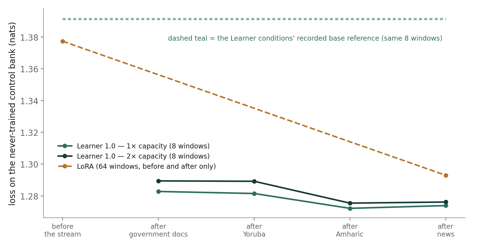
A sequentially trained model can damage text it never trained on. This bank is the check for that.

This control is a small, mostly Amharic bank, scored on 8 windows for Learner 1.0 and on 64 for LoRA. The benchmark evidence for that belongs to the ten-skill study. Holding a slice back before you start lets you run the same check on your own stream.

Replicate it. Receipts and curves for this figure: science/plasticity-without-forgetting in the replication repository

The control was scored on 8 windows for Learner 1.0 and on 64 for LoRA, one run per experiment. All three improved it. Because the samples differ, read each experiment against its own starting value.

What these traits add up to

The program behind Learner 1.0 tracks a fixed list of goals. This experiment speaks to four of them directly.

Stability with plasticity

The central trade every continual-learning method faces is between learning the new thing and keeping the old ones. Figures 1–4 together show Learner 1.0 on the good side of both at once, at either capacity: measured acquisition similar to this capacity-matched LoRA setup, and an end-of-stream change about two orders of magnitude smaller.

Positive backward transfer

Some of the bars sit below zero, which is positive backward transfer: an earlier domain that gets better while the model trains on later ones. In the continual-learning literature this is the sought-after direction, because it means the later material is reusing representations the earlier material built rather than overwriting them. At 1× capacity the first two domains' losses fell (−0.0011 and −0.0012 nats) while the model trained on the domains that followed, and at 2× the first domain fell by 0.0037 nats (Fig. 2). The third domain rose by +0.002 in both. The first domain improved in both Learner conditions after later domains were trained.

The control

The never-trained control (Fig. 7) does not rise under any experiment. It is mostly Amharic text, so it shows that training on the stream did not damage nearby held-out text.

Curve shape

At the first recorded evaluation, 25 steps into each domain, the Learner 1.0 experiments are already close to their eventual loss (Fig. 6). Measured against each domain’s own base reference, that first evaluation already holds 82–125 per cent of the acquisition the rank-matched LoRA reaches after all 300 updates. What the grid cannot resolve is how much of that was produced during those 25 updates rather than before the first evaluation, so the figure is a ceiling on the updates needed, not a measurement of the learning rate inside them.

The method, at the level we can state it

The mechanism is confidential. Learner 1.0's internal mechanism, the specific mathematical machinery that produces the behavior measured above, is reserved. What we publish instead is everything needed to verify the claims: the evaluation protocol and the measured receipts and loss curves for all three experiments.

What can be stated: a fixed set of trainable parameters is added: 1.14 B in the 1× experiment and 2.28 B in the 2× experiment. Beyond that the mechanism is withheld.

Data and protocol

The replication material for this report is in science/plasticity-without-forgetting: the per-experiment measured summaries, the training and held-out loss curves, the record of the LoRA run at 2×10⁻⁴, and every figure on this page with the code that draws it. All 1,296 windows that were trained or measured are in data/ as token ids and decoded text: 300 training and 8 held-out windows for each of the four domains, and the 64-window control. The Yoruba, Amharic, news and control text is third-party material and keeps the terms of its sources. A record of which source document each window was cut from is not available. The LoRA training code is not released.

Citation

Every number in this post traces to a receipt file in the program's analysis record. The plotted values ship beside each figure as a JSON file in figures/, and the per-experiment summaries and curves are in the same study folder.

@misc{learnerplasticity, title = {Plasticity Without Forgetting: Learner 1.0 at two capacities vs capacity-matched LoRA}, note = {Learner Labs technical report, v3} }

1. The domain windows are packaged as fixed 256-token sequences. Every training, held-out and control window is in the repository as token ids and decoded text (see Data and protocol).

Site copy of the technical report. The figures, the code that draws them and the plotted values are in the replication repository.

The same figures, redrawn from the released files

Four of the figures above, redrawn from the released receipts and curves by the replication repository’s own plot code — one command, deterministic, every input hashed in the figure’s sidecar. They are here as a check rather than as new findings: if the published files did not support the pictures the argument rests on, these would not match. The fifth is the raw loss behind the stream figure.

Figure 8. Three conditions trained on the same four-domain stream. All three learn each domain in turn; the difference between them shows up afterwards, in what they keep. The same measurement as Figure 1 above, drawn by the repository’s plot code rather than ours.

Figure 9. The raw per-step training loss behind the smoothed stream figure, for all three conditions on identical axes. This is the one figure here with no counterpart above: it is the unsmoothed loss behind Figure 8, kept so the smoothing can be checked.

Figure 10. Both Learner 1.0 conditions keep the earlier domains within a few thousandths of a nat while LoRA r256 gives back 0.07, 0.06 and 0.03 nats; all three learned each domain by about the same amount. The same measurement as Figure 2 above, drawn by the repository’s plot code rather than ours.

Figure 11. On 8 never-trained control windows the two Learner 1.0 conditions move by about 0.01 nats across the stream and sit about 0.12 nats below their recorded base reference. The figure does not isolate how much of that difference arose inside the displayed stream. The same measurement as Figure 7 above, drawn by the repository’s plot code rather than ours.

Figure 12. Held-out loss while each domain is trained, against the recorded base reference (dashed, value shown). The Learner 1.0 conditions are close to their final level by the first measurement at step 25; the LoRA condition gets there over the 300 steps. All three end each domain at a similar level. The same measurement as Figure 6 above, drawn by the repository’s plot code rather than ours.

Measurement notes

Each trained domain holds out 8 windows of 256 tokens. The never-trained control bank holds 64; the Learner 1.0 experiments were scored on 8 of them after every domain, the LoRA experiment on all 64 before and after the stream. Backward transfer is final loss minus the loss at that domain's last training appearance, on the same windows; a positive number is forgetting.
Acquisition is the loss reduction relative to the recorded base reference, the untrained model's loss on the same windows, for every experiment. The trainable parameter counts are 1.14 billion (1×), 2.28 billion (2×) and 1.11 billion (LoRA, rank 256 on the feed-forward projections).
All experiments train on the same windows in the same domain order, one window per update with no gradient accumulation. No experiment interleaves domains: all three train the four domains strictly one after the other, 300 windows each. The first domain is English-language US government documents.
One run per experiment. The stream is 300 updates per domain, 307,200 tokens in total; the ten-skill study is the long stream.